As part of a recent illumination project in Zemax, I wanted to integrate a mixing polygon tunnel as part of an aspheric lens. This would have the benefit of:
Reducing system complexity, as it would combine two components.
Reduce system cost, as both components could be injection molded as a singular system part.
Minimize peak incoherent irradiance, by making the irradiance uniform.
As this is for a bio-medical application, I was also acutely aware that I have to be cautious with incoherent irradiance values, to not cross the Maximum Permissible Exposure (MPE) thresholds for skin. An observation I made was that it was surprisingly easy to fudge the peak incoherent irradiance value on the detector (in my setup), by changing the detector size and the number of pixels. Ultimately this was due to user error, but it proved an interesting problem to figure out and solve.
Per Zemax knowledge base, there is a trade-off between spatial resolution and energy resolution – and a very reasonable question is “How many pixels should I use for a given detector?”. We ultimately want to converge on a proper SNR that gives accurate and truthful results.
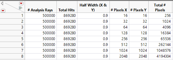
In my case, I was using a source ray file provided by a supplier modeled at 5e5 analysis rays. Setting up my detector at the exit of my mixing tunnel, Zemax tells me that my Total Hits = 869280. I created a JMP data table with different number of X & Y pixels, shown below
To calculate SNR, we need to have a value for signal, and for noise. We divide the total number of rays detected by the total number of pixels, which yields rays per pixel (signal).
A simple noise calculation is SQRT(signal). And our noise % is SQRT(signal)/signal x 100.
Below is the same table, but with additional columns for Rays per Pix (Signal), Noise, and Noise %.
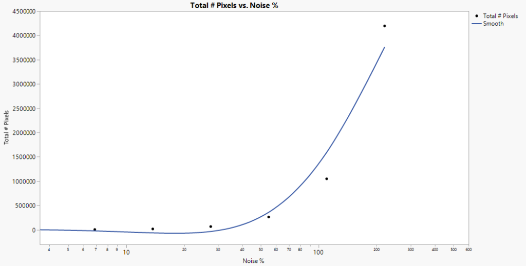
We now have some interesting information to plot. In the first graph, we can see how our noise % increases with total number of pixels, because we have not increased our total number of analysis rays. To me this was not inherently intuitive, as I thought increasing the number of pixels would give me increased spatial resolution. But it turns out that increasing the number of pixels is only part of the solution.
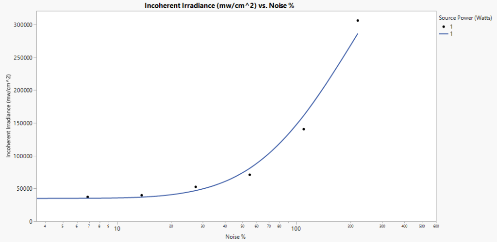
In the second graph, we can really tease out some interesting information. We see that we want to converge on a proper and accurate irradiance value, and that convergence is based on the noise %.
This tells me that for a given detector half-width, and for a given set of analysis rays, it is critical to select a value of pixels for the detector that gives us accurate results.
Finally after calculating and plotting the information above, I can feel confident that I’m presenting an accurate peak irradiance value. The plot shown below was after creating and configuring a merit function to tune the aspheric parameters, and using minimizing standard deviation between pixels as my metric.